
Latent Space Exploration with UMap and Randomized Sparse Mixed Scale Autoencoders
Authors: Eric Roberts and Petrus Zwart
E-mail: PHZwart@lbl.gov, EJRoberts@lbl.gov ___
This notebook highlights some basic functionality with the pyMSDtorch package.
We will setup randomly connected, sparse mixed-scale inspired autoencoders with for unsupervised learning, with the goal of exploring the latent space it generates. These autoencoders deploy random sparsely connected convolutions and random downsampling/upsampling operations (maxpooling/transposed convolutions) for compressing/expanding data in the encoder/decoder halves. This random layout supplants the structured order of typical Autoencoders, which consist downsampling/upsampling operations following dual convolutions.
Like the preceding sparse mixed-scale networks (SMSNets), there exist a number of hyperparameters to tweak so we can control the number of learnable parameters these sparsely connected networks contain. This type of control can be beneficial when the amount of data on which one can train a network is not very voluminous, as it allows for better handles on overfitting. ___
[1]:
import numpy as np

import torch
import torch.nn as nn
import torch.optim as optim

from pyMSDtorch.core import helpers
from pyMSDtorch.core import train_scripts
from pyMSDtorch.core.networks import SparseNet
from pyMSDtorch.test_data.twoD import random_shapes
from pyMSDtorch.core.utils import latent_space_viewer
from pyMSDtorch.viz_tools import plots, draw_sparse_network

import matplotlib.pyplot as plt
from torch.utils.data import DataLoader, TensorDataset
import einops
import umap
Create Data
Using our pyMSDtorch in-house data generator, we produce a number of noisy “shapes” images consisting of single triangles, rectangles, circles, and donuts/annuli, each assigned a different class. In addition to augmenting with random orientations and sizes, each raw, ground truth image will be bundled with its corresponding noisy and binary mask.
Parameters to toggle:
n_train – number of ground truth/noisy/label image bundles to generate for training
n_test – number of ground truth/noisy/label image bundles to generate for testing
noise_level – per-pixel noise drawn from a continuous uniform distribution (cut-off above at 1)
N_xy – size of individual images
[2]:
N_train = 500
N_test  = 15000
noise_level = 0.50
Nxy = 32

train_data = random_shapes.build_random_shape_set_numpy(n_imgs=N_train,
                                                        noise_level=noise_level,
                                                        n_xy=Nxy)
test_data = random_shapes.build_random_shape_set_numpy(n_imgs=N_test,
                                                       noise_level=noise_level,
                                                       n_xy=Nxy)

test_GT = torch.Tensor(test_data["GroundTruth"]).unsqueeze(1)
View shapes data
[3]:
plots.plot_shapes_data_numpy(train_data)
Dataloader class
Here we cast all images from numpy arrays and the PyTorch Dataloader class for easy handling and iterative loading of data into the networks and models.
[4]:
which_one = "Noisy" #"GroundTruth"

batch_size = 100

loader_params = {'batch_size': batch_size,
                 'shuffle': True}
Ttrain_data = TensorDataset( torch.Tensor(train_data[which_one]).unsqueeze(1) )

train_loader = DataLoader(Ttrain_data, **loader_params)

loader_params = {'batch_size': batch_size,
                 'shuffle': False}
Ttest_data = TensorDataset( torch.Tensor(test_data[which_one][0:N_train]).unsqueeze(1) )
test_loader = DataLoader(Ttest_data, **loader_params)

Tdemo_data = TensorDataset( torch.Tensor(test_data[which_one]).unsqueeze(1) )
demo_loader = DataLoader(Tdemo_data, **loader_params)
Build Autoencoder
There are a number of parameters to play with that impact the size of the network:
latent_shape: the spatial footprint of the image in latent space. I don’t recommend going below 4x4, because it interferes with the dilation choices. This is a bit of a bug, we need to fix that. Its on the list.
out_channels: the number of channels of the latent image. Determines the dimension of latent space: (channels,latent_shape[-2], latent_shape[-1])
depth: the depth of the random sparse convolutional encoder / decoder
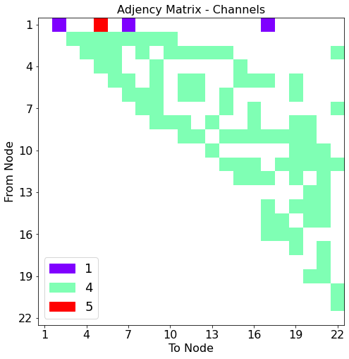
hidden channels: The number of channels put out per convolution.
max_degree / min_degree : This determines how many connections you have per node.
Other parameters do not impact the size of the network dramatically / at all:
in_shape: determined by the input shape of the image.
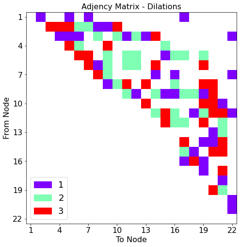
dilations: the maximum dilation should not exceed the smallest image dimension.
alpha_range: determines the type of graphs (wide vs skinny). When alpha is large,the chances for skinny graphs to be generated increases. We don’t know which parameter choice is best, so we randomize it’s choice.
gamma_range: no effect unless the maximum degree and min_degree are far apart. We don’t know which parameter choice is best, so we randomize it’s choice.
pIL, pLO, IO: keep as is.
stride_base: make sure your latent image size can be generated from the in_shape by repeated division of with this number.
[19]:
autoencoder = SparseNet.SparseAutoEncoder(in_shape=(32, 32),
                                          latent_shape=(4, 4),
                                          depth=20,
                                          dilations=[1,2,3],
                                          hidden_channels=4,
                                          out_channels=1,
                                          alpha_range=(0.05, 0.25),
                                          gamma_range=(0.0, 0.5),
                                          max_degree=10, min_degree=4,
                                          pIL=0.15,
                                          pLO=0.15,
                                          IO=False,
                                          stride_base=2)
pytorch_total_params = helpers.count_parameters(autoencoder)
print( "Number of parameters:", pytorch_total_params)
Number of parameters: 89451
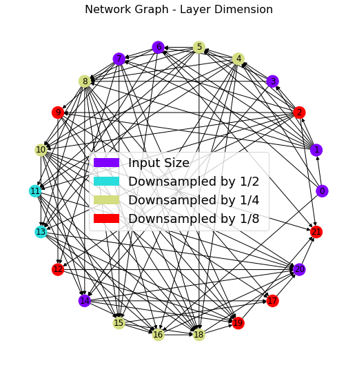
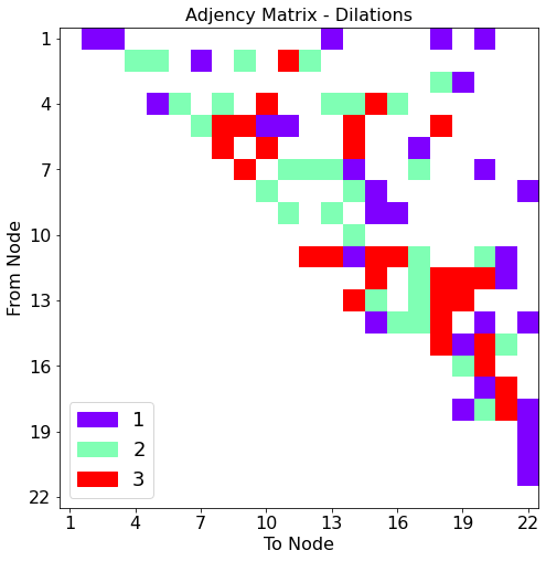
We visualize the layout of connections in the encoder half of the Autoencoder, the first half responsible for the lower-dimensional compression of the data in the latent space.
[20]:
ne,de,ce = draw_sparse_network.draw_network(autoencoder.encode)
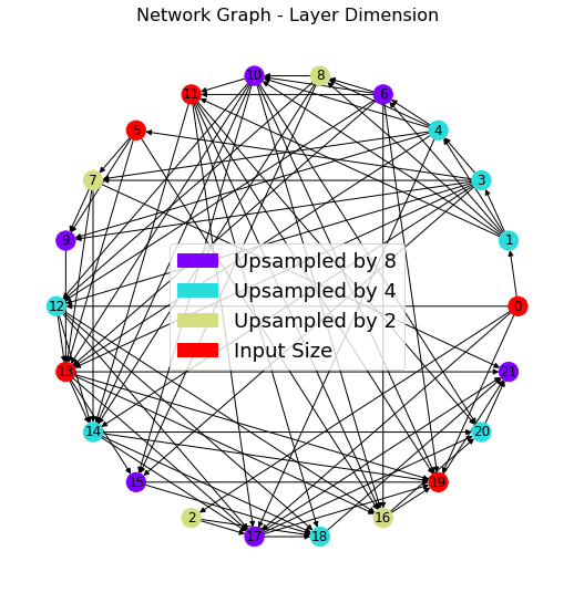
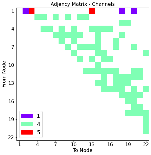
Now the visualization of connections comprising the decoder half of the Autoencoder. This second half is responsible for reconstructing the exact image input from the compressed information in the latent space
[21]:
nd,dd,cd = draw_sparse_network.draw_network(autoencoder.decode)
Training the Autoencoder
Training hyperparameters are specified.
[ ]:
torch.cuda.empty_cache()   # Empty superfluous information from GPU memory

learning_rate = 1e-3
num_epochs=25
criterion = nn.L1Loss()
optimizer = optim.Adam(autoencoder.parameters(), lr=learning_rate)
[22]:
torch.cuda.empty_cache()
learning_rate = 1e-3
num_epochs=25
criterion = nn.L1Loss()
optimizer = optim.Adam(autoencoder.parameters(), lr=learning_rate)
rv = train_scripts.train_autoencoder(net=autoencoder.to('cuda:0'),
                               trainloader=train_loader,
                               validationloader=test_loader,
                               NUM_EPOCHS=num_epochs,
                               criterion=criterion,
                               optimizer=optimizer,
                               device="cuda:0", show=1)
print("Best Performance:", rv[1]["CC validation"][rv[1]['Best model index']])
Epoch 1 of 25 | Learning rate 1.000e-03
Training Loss: 4.2694e-01 | Validation Loss: 3.8143e-01
Training CC: -0.0337   Validation CC  : -0.0311
Epoch 2 of 25 | Learning rate 1.000e-03
Training Loss: 3.7770e-01 | Validation Loss: 3.4278e-01
Training CC: 0.0115   Validation CC  : 0.0710
Epoch 3 of 25 | Learning rate 1.000e-03
Training Loss: 3.4378e-01 | Validation Loss: 3.1645e-01
Training CC: 0.1143   Validation CC  : 0.1622
Epoch 4 of 25 | Learning rate 1.000e-03
Training Loss: 3.1984e-01 | Validation Loss: 2.9729e-01
Training CC: 0.2002   Validation CC  : 0.2451
Epoch 5 of 25 | Learning rate 1.000e-03
Training Loss: 3.0146e-01 | Validation Loss: 2.8159e-01
Training CC: 0.2832   Validation CC  : 0.3263
Epoch 6 of 25 | Learning rate 1.000e-03
Training Loss: 2.8595e-01 | Validation Loss: 2.6843e-01
Training CC: 0.3553   Validation CC  : 0.3836
Epoch 7 of 25 | Learning rate 1.000e-03
Training Loss: 2.7259e-01 | Validation Loss: 2.5695e-01
Training CC: 0.4126   Validation CC  : 0.4439
Epoch 8 of 25 | Learning rate 1.000e-03
Training Loss: 2.6081e-01 | Validation Loss: 2.4615e-01
Training CC: 0.4717   Validation CC  : 0.4990
Epoch 9 of 25 | Learning rate 1.000e-03
Training Loss: 2.4975e-01 | Validation Loss: 2.3617e-01
Training CC: 0.5263   Validation CC  : 0.5514
Epoch 10 of 25 | Learning rate 1.000e-03
Training Loss: 2.3939e-01 | Validation Loss: 2.2670e-01
Training CC: 0.5776   Validation CC  : 0.5999
Epoch 11 of 25 | Learning rate 1.000e-03
Training Loss: 2.2954e-01 | Validation Loss: 2.1779e-01
Training CC: 0.6233   Validation CC  : 0.6419
Epoch 12 of 25 | Learning rate 1.000e-03
Training Loss: 2.1994e-01 | Validation Loss: 2.0904e-01
Training CC: 0.6645   Validation CC  : 0.6801
Epoch 13 of 25 | Learning rate 1.000e-03
Training Loss: 2.1043e-01 | Validation Loss: 2.0099e-01
Training CC: 0.7017   Validation CC  : 0.7139
Epoch 14 of 25 | Learning rate 1.000e-03
Training Loss: 2.0229e-01 | Validation Loss: 1.9438e-01
Training CC: 0.7325   Validation CC  : 0.7398
Epoch 15 of 25 | Learning rate 1.000e-03
Training Loss: 1.9486e-01 | Validation Loss: 1.8969e-01
Training CC: 0.7568   Validation CC  : 0.7586
Epoch 16 of 25 | Learning rate 1.000e-03
Training Loss: 1.8991e-01 | Validation Loss: 1.8624e-01
Training CC: 0.7744   Validation CC  : 0.7740
Epoch 17 of 25 | Learning rate 1.000e-03
Training Loss: 1.8582e-01 | Validation Loss: 1.8289e-01
Training CC: 0.7885   Validation CC  : 0.7875
Epoch 18 of 25 | Learning rate 1.000e-03
Training Loss: 1.8229e-01 | Validation Loss: 1.7995e-01
Training CC: 0.8005   Validation CC  : 0.7982
Epoch 19 of 25 | Learning rate 1.000e-03
Training Loss: 1.7943e-01 | Validation Loss: 1.7751e-01
Training CC: 0.8101   Validation CC  : 0.8064
Epoch 20 of 25 | Learning rate 1.000e-03
Training Loss: 1.7690e-01 | Validation Loss: 1.7544e-01
Training CC: 0.8176   Validation CC  : 0.8127
Epoch 21 of 25 | Learning rate 1.000e-03
Training Loss: 1.7452e-01 | Validation Loss: 1.7337e-01
Training CC: 0.8236   Validation CC  : 0.8181
Epoch 22 of 25 | Learning rate 1.000e-03
Training Loss: 1.7302e-01 | Validation Loss: 1.7147e-01
Training CC: 0.8283   Validation CC  : 0.8227
Epoch 23 of 25 | Learning rate 1.000e-03
Training Loss: 1.7083e-01 | Validation Loss: 1.6990e-01
Training CC: 0.8332   Validation CC  : 0.8273
Epoch 24 of 25 | Learning rate 1.000e-03
Training Loss: 1.6946e-01 | Validation Loss: 1.6901e-01
Training CC: 0.8374   Validation CC  : 0.8306
Epoch 25 of 25 | Learning rate 1.000e-03
Training Loss: 1.6766e-01 | Validation Loss: 1.6728e-01
Training CC: 0.8411   Validation CC  : 0.8342
Best Performance: 0.8341745018959046
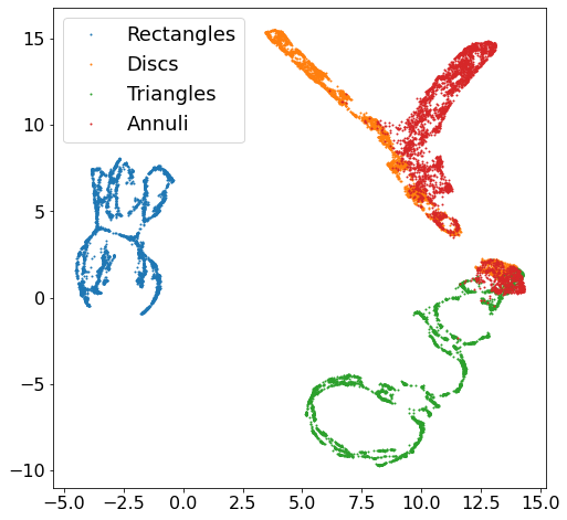
Latent space exploration
With the full SMSNet-Autoencoder trained, we pass new testing data through the encoder-half and apply Uniform Manifold Approximation and Projection (UMap), a nonlinear dimensionality reduction technique leveraging topological structures.
Test images previously unseen by the network are shown in their latent space representation.
[23]:
results = []
latent = []
for batch in demo_loader:
    with torch.no_grad():
        res = autoencoder(batch[0].to("cuda:0"))
        lt = autoencoder.latent_vector(batch[0].to("cuda:0"))
        results.append(res.cpu())
        latent.append(lt.cpu())
results = torch.cat(results, dim=0)
latent = torch.cat(latent, dim=0)
[24]:
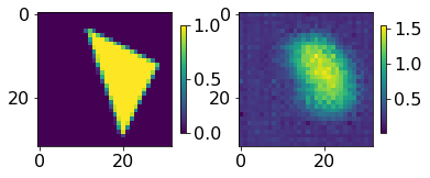
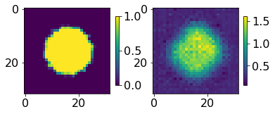
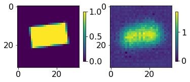
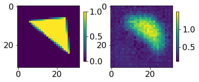
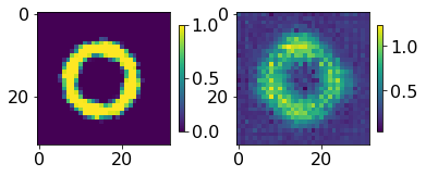
for ii,jj in zip(test_GT.numpy()[0:5],results.numpy()[0:5]):
    fig, axs = plt.subplots(1,2)
    im00 = axs[0].imshow(ii[0,...])
    im01 = axs[1].imshow(jj[0])
    plt.colorbar(im00,ax=axs[0], shrink=0.45)
    plt.colorbar(im01,ax=axs[1], shrink=0.45)
    plt.show()
    print("-----------------")
-----------------
-----------------
-----------------
-----------------
-----------------
Autoencoder latent space is further reduced down to two dimensions; i.e. each image passed though the encoder is represented by an integer pair of coordinates below, with blue repesenting all rectangles, orange representing all circles/discs, green representing all triangles, and red representing all annuli.
[25]:
umapper = umap.UMAP(min_dist=0, n_neighbors=35)
X = umapper.fit_transform(latent.numpy())
[26]:
these_labels = test_data["Label"]
plt.figure(figsize=(8,8))
for lbl in [1,2,3,4]:
    sel = these_labels==lbl
    plt.plot(X[sel,0], X[sel,1], '.', markersize=2)
plt.legend(["Rectangles","Discs","Triangles","Annuli"])
plt.show()
Below simply averages all nearest-neighbors for visualization purposed.
[27]:
fig = latent_space_viewer.build_latent_space_image_viewer(test_data["GroundTruth"],
                                X,
                                n_bins=50,
                                min_count=1,
                                max_count=1,
                                mode="mean")
[ ]: